Tutorial, Part 3

Here, in Part 3, we will customize the project to:

• modify chart appearance,
• add another query and plot the results, and
• aggregate regions to simplify plot appearance.

3.0 The chart sub-command

The chart sub-command plots data provided in CSV files. A typical workflow is to run queries on GCAM results to produce CSV files, compute differences and then use chart to plot any or all of this. If you compute custom results, you can store in CSV files as well, and use chart on those.

The chart sub-command offers numerous options to control the appearance of figures. Take a moment to review this using the link above.

We need to refer to the project file for the tutorial, so we’ll present it again here:

<?xml version="1.0" encoding="UTF-8"?>
<!--
This file defines the "tutorial" project. Feel free to edit it to your liking.
Also see project2.xml, which offers a slightly more complex example.
-->
<projects xmlns:xsi="http://www.w3.org/2001/XMLSchema-instance"
          xsi:noNamespaceSchemaLocation="project-schema.xsd">
  <project name="ctax">
    <vars>
      <var name="startYear">2015</var>
      <var name="endYear">2050</var>  <!-- stops at 2050 so tutorial runs faster -->
      <var name="years" eval="1">{startYear}-{endYear}</var>
    </vars>
    <steps>
      <!--
      The names defined in steps can be used on the command-line to limit operations to
      these steps. Steps are run in the order defined in this file, regardless of the
      order specified to "gt run". If runFor="baseline", the step is run only for baseline
      scenarios. If runFor="policy", the step is run only for non-baseline scenarios. If
      not set (or set to any other value) the step is run for all scenarios.
       -->
      <step name="setup" runFor="baseline">
        @setup -b "{baseline}" -g "{scenarioGroup}" -S "{scenarioSubdir}" -w "{scenarioDir}"
               -p {endYear} -y {years}
      </step>
      <step name="gcam"  runFor="baseline">@gcam -s "{baseline}" -S "{projectXmlDir}"</step>
      <step name="query" runFor="baseline">
        @query -o "{batchDir}" -w "{scenarioDir}" -s "{scenario}" -q "{queryXmlFile}"
      </step>

      <!--
        Explicitly require policy setup, gcam, and query steps to run after baseline to
        allow baseline results to be used in constraints
      -->
      <step name="setup" runFor="policy">
            @setup -b "{baseline}" -s "{scenario}" -g {scenarioGroup} -S "{scenarioSubdir}"
                   -w "{scenarioDir}" -p {endYear} -y {years}
      </step>
      <step name="gcam"  runFor="policy">@gcam -s "{scenario}" -S "{projectXmlDir}"</step>
      <step name="query" runFor="policy">
        @query -o {batchDir} -w "{scenarioDir}" -s "{scenario}" -q "{queryXmlFile}"
      </step>

      <!--
        Compute and plot differences between query results for policy and baseline scenarios
      -->
      <step name="diff"  runFor="policy">
        @diff -D "{sandboxDir}" -y {years} -q "{queryXmlFile}" "{baseline}" "{scenario}"
      </step>
      <step name="plotDiff" runFor="policy">
        @chart {diffPlotArgs} --reference "{baseline}" --scenario "{scenario}" --fromFile "{diffPlots}"
      </step>

      <!-- Generate an XLSX workbook from all CSV query result files -->
      <step name="xlsx"  runFor="policy">
        @diff -D "{diffsDir}" -c -y {years} -o diffs.xlsx {diffsDir}/*.csv
      </step>
    </steps>

    <!--
      Define which queries to run. This creates a text file whose name is stored
      in a project variable, accessed as {queryXmlFile} in the "query" step.
    -->
    <queries varName="queryXmlFile">
      <query name="LUC_emissions_by_region"/>
      <query name="total_climate_forcing"/>
      <query name="global_mean_temperature"/>
    </queries>

    <vars>
      <!-- common arguments for 'diffPlots' -->
      <var name="diffPlotArgs" eval="1">-D "{diffsDir}" --outputDir figures --years {years} --label --ygrid --zeroLine</var>
    </vars>

    <tmpFile varName="diffPlots">
      <text>LUC_emissions_by_region-{scenario}-{reference}.csv -Y 'Tg CO$_2$' -m C_to_CO2 -i -n 4 -T '$\Delta$ LUC emissions' -I region -x by-region.png</text>

      <!-- Forcing and temperature change -->
      <text>total_climate_forcing-{scenario}-{reference}.csv   -Y 'W/m$^2$' --timeseries -T '$\Delta$ Total Climate Forcing'</text>
      <text>global_mean_temperature-{scenario}-{reference}.csv -Y 'Degrees C' --timeseries -T '$\Delta$ Global Mean Temperature'</text>
    </tmpFile>

  </project>
</projects>

Notice the following:

• Line 50 defines <step name="plotDiff" runFor="policy">, which calls the internal @chart sub-command.

• The @chart command references 4 variables in curly braces: {diffPlotArgs}, {diffPlots}, {baseline}, and {scenario}.

• {diffPlotArgs} and {diffPlots} are defined later in the project file (at lines 72 and 75, respectively) while {baseline} and {scenario} are defined internally by the run command.

• The variable diffPlotArgs provides some options for the chart command that are common to our charts. Consolidating them here allows us to control aesthetics more easily. The following options used are:

  -D {diffsDir} --outputDir figures --years {years} --label --ygrid --zeroLine
  

Where:

• -D {diffsDir} indicates the directory in which files are found. The value {diffsDir} is filled in at run-time, since it differs for each scenario.
• --outputDir figures indicates that plots should be written in the directory figures, relative to the directory specified with -D.
• --years {years} says to plot results for this range of years. The value for {years} is defined at line 12. This is defined in a variable to allow the range to be changed consistently for all plots by changing either the start or end years, defined at lines 10 and 11, which in turn form the value for years
• --label requests that a label be rendered down the right side of the figure with the name of the file.
• ygrid requests that light grey horizontal lines at major Y-axis values.
• --zeroLine requests a line drawn at zero on all figures

Lines 75-81, starting with <tmpFile varName="diffPlots"> defines a temporary file whose contents are composed from the enclosed <text> elements, and whose name is stored in the project variable named diffPlots. (Temporary files are deleted before GCAM tool (gt) exits.) The chart sub-command can be passed the name of a file containing options defining a plot to create, one plot per line. The options on each line of this file are combined with those at the command-line level (in this case via {diffPlotArgs}. This is complicated, but it reduces a lot of redundancy.

CSV files generated by queries include the name of the query (with spaces replaced by hyphens) followed by a hyphen and the scenario name. CSV files generated by the diff sub-command have a similar convention, but the name includes both the scenario and baseline names, separated by a hyphen. Thus, the results from the difference file created by running the query titled “Land Use Change Emission” on both the baseline and policy and subtracting, is called:

Land_Use_Change_Emission-{scenario}-{reference}.csv

3.1 Modify plot appearance

We will now modify the plot slightly. Let’s:

• make the label black, rather than light grey
• add a box around the plot
• remove the grid lines
• remove the zero line

We do this by changing the definition of plotDiffArgs to this:

<var name="diffPlotArgs" eval="1">-D {diffsDir} --outputDir figures --years {years} --label --labelColor=black --box</var>

To regenerate the figure for the tax-10 scenario, run this command:

$ gt run -S tax-10 -s plotDiff

The Land Use Change Emissions plot now looks like this:

---

---

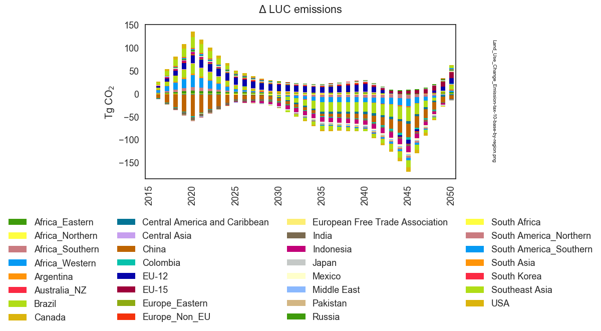
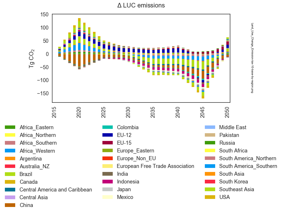
Let’s also change the number of columns in the legend by changing -n 4 on line 76 to -n 3, so the legend isn’t quite so wide. Run the plotDiff step again, as above. We now see:

---

---

In Tutorial, Part 4, we will modify our queries to aggregate into a smaller number of regions.